


Preamble
Last week we wrote about attempts to measure the economy and we highlighted two pioneers of cross-country comparisons, Michael Mulhall and Angus Maddison. We also had a brief look at what the (very) long-run picture of economic growth looked like using the widely used Maddison database.
This time we’re looking at economic growth over the past 50 years. The biggest story is the rise of China. But how fast and how big has this been?
We were motivated by some suspicious-looking figures for China when we were looking at energy intensity – energy use per unit of GDP – in the historical record. It turns out the anomaly had nothing to do with the numerator (energy use) and everything to do with the denominator (GDP) when the source was the latest release of the Penn World Tables (PWT) – version 11.
PWT is one of the most widely used databases in economics – the required Feenstra et al. (2015) citation for PWT has over 8000 cites according to Google Scholar. PWT has been around since the 1980s and collects internationally comparable macroeconomic data. Usually with the release of such a widely-used international database there is just an extension to the database, a change in the price base, some changes to historical series that don’t affect the big picture, and maybe an increase in coverage, but this time was different.
Some background history on comparative national accounts
One of the biggest, and oldest, questions in economics is why are some countries rich and others poor. Adam Smith set about addressing this question in An Inquiry into the Nature and Causes of the Wealth of Nations 250 years ago. But before we can explain differences in national prosperity, we first have to measure the differences in national income. Comparing national incomes across countries is harder than it sounds. It requires converting different currencies into a common unit while accounting for differences in prices, consumption patterns (colder countries are going to need more central heating, hotter countries consume more air conditioning, and what do we do about public versus private health care systems?), and also the large share of goods and services that are not internationally traded (e.g., haircuts or funeral services).
The British-Australian economist Colin Clark was one of the first economists to confront this problem systematically. In his 1940 book Conditions of Economic Progress, Clark introduced an ‘international unit’ (I.U.) to compare real incomes across countries with different price levels and consumption patterns. Defined relative to the US dollar as ‘the amount of goods and services which could be purchased for $1 in the US’, the international unit provided one of the first practical ways of comparing living standards across countries. His estimates revealed a striking divide between industrial and non-industrial economies and led him to conclude that the world was ‘a wretchedly poor place’. Clark found that the United States had the highest level of income per worker, with the United States, Canada and New Zealand each exceeding $1,000 I.U., while China and India had much lower figures of $120 and $200 I.U., respectively. This is a useful benchmark for our discussion below.
Further progress in international comparability came from the Irish statistician Roy Geary (1958), whose work was later refined by the Palestinian economist Salem Khamis (1984). Geary, while working as a consultant for the FAO in the 1950s, devised an international unit of comparison that was subsequently formalized by Khamis. The aim was to compare national incomes using a common numeraire, thereby avoiding distortions from exchange rates. This approach became known as the Geary–Khamis international dollar – this was the unit of measurement, 1990 Geary-Khamis dollars, used by Angus Maddison (2001).
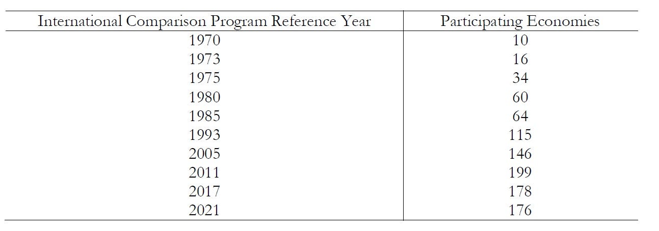
Today, cross-country comparisons are usually based on purchasing power parities (PPPs), which construct conversion rates designed to equalise the purchasing power of currencies across economies. PPP exchange rates have been collected in large-scale international surveys. The International Comparison Project (now called the International Comparison Program) started in 1968, with the first comparison carried out in 1970. It subsequently became the basis of prices underpinning PPP adjustments. As Angus Deaton (2010) dryly observed, the ICP exercises were ‘like the Olympics’ because they occurred infrequently and there were very few participants in initial rounds of these exercises; this has increased over time from 10 countries in 1970, to 60 countries in 1980, to 199 in 2011.
Rounds of the ICP and participating economics, 1970-2021
The Penn World Tables
Systematic estimates of internationally comparable real incomes were developed through a cross-country project initiated by Robert Summers, Irving Kravis and Alan Heston in the 1970s (Kravis et al. 1975). The result became one of the foundational datasets of modern empirical macroeconomics, underpinning research on growth, convergence, productivity and the sources of international income differences (e.g., Mankiw et al. 1992; Jones & Romer 2010); it is also widely used in classrooms to teach economic growth.
Summers, Kravis, and Heston were associated with the University of Pennsylvania, and their project became known as The Penn World Tables (PWT). The motivation for the study was the ‘unsatisfactory procedures generally followed in the past’ whereby cross-country comparisons were being based on nominal (current) prices and not constant prices (Summers et al. 1980). The data was in real terms building on ICP that was undertaken by Summers, Kravis and Heston working with the World Bank.
The original database (PWT 1) contained real GDP, real consumption, and real fixed capital formation for 119 countries in 1950 and from 1960 to 1977. Subsequent updates of the PWT included more variables and more time periods. For example, PWT 4 contained data on 17 variables (and 2 variables for centrally planned economies) for 130 countries; it was PWT 4 that was used in one of the early empirical studies on economic growth (Mankiw et al. 1992). PWT 5 contained data on 27 variables from 1950 to 1985 for 138 countries, including the necessary data to compare productivity across countries. Version 8 of the PWT moved to the University of California, Davis and the University of Groningen but retained the Penn trademark. The updated PWT includes estimates of total factor productivity and capital stocks across countries. Other well-known sources of macroeconomic data, such as the World Bank’s World Development Indicators and The Conference Board, basically align with the PWT and can effectively be used interchangeably.
The latest Penn World Tables
In October 2025, PWT 11 was released without much fanfare. It incorporated new PPP benchmarks and updated national accounts, but one methodological change is particularly consequential: the treatment of China (see Inklaar and Gräler, What is new in PWT 11.0). A major revision to the PWT methodology replaced the earlier adjusted GDP estimates for China with China’s official national accounts and incorporated new PPP estimates and updated human-capital and labour-share measures. This history matters because the Penn World Table is not simply a repository of official statistics. Its purpose has always been to make difficult methodological choices in pursuit of internationally comparable measures of real economic performance. With PWT 11, one of those choices has changed dramatically and it has resulted in a new statistical history of Chinese growth.
How big was China?
The revision to the China GDP series in PWT 11 is discussed at length by Inklaar and Gräler. Prior to the latest revision, the PWT series China relied heavily on an alternative GDP series constructed by Harry Wu (2014), and and earlier adjustment that Wu made when working with Angus Maddison (2008). This work was motivated by concerns that the official Chinese data were overstating economic growth. Inklaar and Gräler summarise the adjustments Wu and Maddison make as (1) revising downwards labour productivity growth in services sectors, and (2) using a different weighting scheme for an index of industrial production. PWT 11 drops this approach and switches to using the official Chinese GDP series.
As Inklaar and Gräler note, this makes a big difference. The figure below is a modified version of one that appears in the PWT 11 documentation.1 PWT provide several real GDP series; we use the ‘national accounts’ (‘na’) series here. We report the previous edition of PWT, 10.01, along with the new 11.0 and, for reference, the series from the Maddison Project (see part 1 of this series). The Maddison Project data also use the Maddison-Wu approach, and so will track PWT 10 closely.
China real GDP, 1952=1 (log scale)
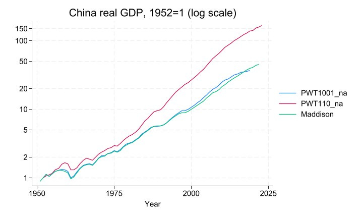
The data start with GDP indexed to 1 in 1952. In 2019, the last year for which we have data for all 3 series, Chinese GDP is 37 times bigger than in 1952 according to PWT 10, 39 times bigger according to the Maddison Project, and whopping 138 times bigger according to PWT 11.
This is a huge difference: in log terms, GDP growth was about 5.5% p.a. according to Maddison-Wu and the previous edition of PWT vs. 7.2% p.a. using the official data. The impact is bigger still when looking at the reform period: between 1977 (the last year before reforms started) and 2019, GDP grew by 6.2-6.4% p.a. according to the old methodology, and 8.8% p.a. according to official data. This translates mechanically to an upwards revision of about 2.5% p.a. in China’s TFP growth. A massive acceleration in the growth rate of over 1/3.
But how plausible is this? Thanks to improvements in the collection of statistics and the efforts of the ICP, we have a pretty good idea of how big the Chinese economy is now, and the PWT revisions didn’t change this much: according to PWT 10, in 2019 the Chinese and US economies were about the same size, and in the revised PWT 11 data China was about 13% bigger. Small beer by comparison.
The plausibility or otherwise of the new series rests, rather, on how big the Chinese economy was in 1952 or 1977. That is, instead of the figure on the left, we should consider the figure on the right.
China real GDP, 1950-2023 (log scale)
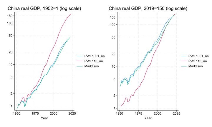
The only difference is that we set the benchmark to 2019, and we ask whether the revision to Chinese GDP in 1952 or 1977 is plausible. How reasonable is it to revise Chinese living standards downwards by a factor of about 4 in 1952 and about 3 in 1977?
We think the answer is … not very, and simply because the implied standard of living is too low to be believed. The simplest way to illustrate this is to compare China with other countries in these earlier years. Here we compare Chinese GDP per capita to that in 3 other major Asian economies: India, South Korea, and Japan. To show that this is a fundamental problem and doesn’t depend on any particular definition of GDP, we report 9 different series.
Five series rely on the official growth rate: the two PWT 11 series (the ‘na’ series and GDP by origin, the ‘o’ series), The Conference Board (TCB) main series, the World Bank’s World Development Indicators (WDI) series in purchasing power parity (PPP), and the University of Queensland UQICD series. Four series use the Wu/Maddison-Wu approach: the two PWT 10 series, the Maddison Project (of course), and The Conference Board’s alternative TCB2 series. We have normalised so all series are in approx. 2017 prices.
GDP per capita, 1950-2023 (log scale)
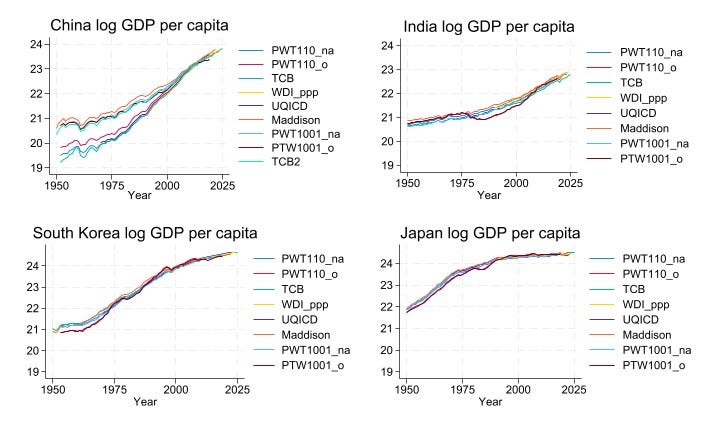
The level and path of development for India, South Korea and Japan are pretty consistent across all sources. The key feature to note from the pictures is the starting point. Japan had started industrialising many years before the others, and this is apparent in the data (using the Maddison series, Japan’s GDP per capita in 1952 was not quite 4x than in India or South Korea). India and South Korea were both still very poor and agricultural in 1952. We would expect the standard of living in China to be similar, and this is what the pre-revision PWT and other Maddison-Wu data show. But the new PWT data suggest that China was incredibly poor: about 3x poorer India and 5x poorer (!) than South Korea. Really?
Or we can look at the poorest countries in the world in 1977, the year before the Deng reforms began. According to PWT 10, China was the 24th-poorest country in the world, slightly richer than Laos (22nd), India (20th) and Vietnam (19th). Very plausible in cross-country comparison. But in PWT 11, China is the 2nd-poorest country in the world!? The poorest is Mali; countries just above China in the ranking are Mozambique, Somalia, Rwanda, Ethiopia…. And India is almost 3x richer in 1977. Really?
Other evidence that China did not belong in the deeply-poor group in 1977 is readily available. The table below reports UN infant mortality and crude death rate figures, and PWT 11’s own human capital index (based on years of schooling), for the aforementioned comparator countries for 1977.
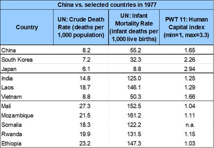
China clearly does not belong in the deeply-poor group, whatever indicator is used. It is hard to avoid the conclusion that the appearance of deep poverty in 1977 and earlier is an artefact of extrapolating backwards using an overstated growth rate.
Interestingly, Inklaar and Gräler are well aware of this line of argument, and discuss it explicitly in the context of past PWT choices for how to deal with Chinese data. At the end of their summary of the thinking that went into PWT 11, they write ‘The argument that extrapolating Chinese GDP levels over a long period of time implies unrealistically low income levels remains a concern. But here too, China’s data are not unique. … Evidence … suggests that many countries overstate growth, making it difficult to justify singling out China.’2
We beg to differ. Just because it’s a potential problem for other countries is not a compelling reason to make the same mistake for what is now the biggest economy in the world (according to the CIA before they stopped publishing their World Factbook (McLaughlin 2026)), and the single biggest driver behind the decline of poverty worldwide in the last half-century.
Fortunately, the old PWT/Maddison-Wu methodology is being maintained by The Conference Board, so researchers interested in long-run growth have a ready alternative.
Summary
What does it all mean? Well, we know that China is now the largest economy in the world (that is according to PWT). But we are unsure exactly how it got there. In earlier iterations of the PWT China’s growth record since the 1950s has been driven primarily by capital accumulation rather than improvements in productivity.
That was the conventional story, but the PWT 11 changes substantially raised China’s measured real GDP growth and, as a consequence, its implied TFP growth. In PWT 11, China’s TFP growth since the 1980s is much stronger and China’s TFP performance at times approaches or even surpasses that of the United States. This just highlights how sensitive TFP measurement can be. The longstanding concerns over China’s official GDP estimates therefore remain. While the shift in PWT methodology eliminates earlier downward adjustments, it does not resolve the underlying measurement challenges.
References
Clark, C. (1940). The Conditions of Economic Progress. London: Macmillan.
Deaton, A. (2010). Measuring Development: Different Data, Different Conclusions? In Measure for Measure – How Well Do We Measure Development? Proceedings of the 8th AFDEUDN Conference.
Feenstra, Robert C., Robert Inklaar and Marcel P. Timmer (2015). The Next Generation of the Penn World Table. American Economic Review, 105(10), 3150-3182
Geary, R. C. (1958). A Note on the Comparison of Exchange Rates and Purchasing Power Between Countries. Journal of the Royal Statistical Society. Series A, 121(1): 97–9.
Jones, C. I. and Romer, P. M. (2010). The New Kaldor Facts: Ideas, Institutions, Population, and Human Capital. American Economic Journal: Macroeconomics, 2:1, 224–245
Khamis, S. H, (1984). On Aggregation Methods for International Comparisons. Review of Income and Wealth, 30(2): 185-205.
Kravis, I. B., Kenessey, Z., Heston, A. and Summers, R. (1975). A System of International Comparisons of Gross Product and Purchasing Power. Baltimore: John Hopkins Press.
Maddison, A. (2001). The World Economy: A Millennial Perspective. Paris: OECD.
Maddison, A. and Wu, H. X. (2008). Measuring China’s Economic Performance. World Economics, Vol. 9 (2).
Mankiw, N. G., Romer, D., and Weil, D. N. (1992). A Contribution to the Empirics of Economic Growth. The Quarterly Journal of Economics, 107(2):407–37.
McLaughlin, E. (2026). The Inclusive Wealth of Nations. Prosperity, Sustainability, and the Future of Economic Progress. London: Bloomsbury.
Pandian, R. K. (2025). Overstatement of GDP growth in autocracies and the recent decline in global inequality. Social Forces, 104(1), 90-111.
Summers, R., Kravis, I. B., and Heston, A. (1980). International Comparisons of Real Product and Its Composition: 1950–77. Review of Income and Wealth, 26(1): 19–33.
Wu, H. X. (2014). China’s Growth and Productivity Performance Debate Revisited: Accounting for China’s Sources of Growth with A New Data Set. The Conference Board Economics Program Working Paper Series, 14-01
The figure that appears in the PWT documentation contrasts the Wu series for total GDP with an official series based on data from the UN and the World Bank.
This view is also consistent with recent evidence that growth may be systematically overstated in many autocratic countries (e.g. Pandian 2025).